betaParamsFromQuantiles

library(BetaBayes)
library(ggplot2)

Use case

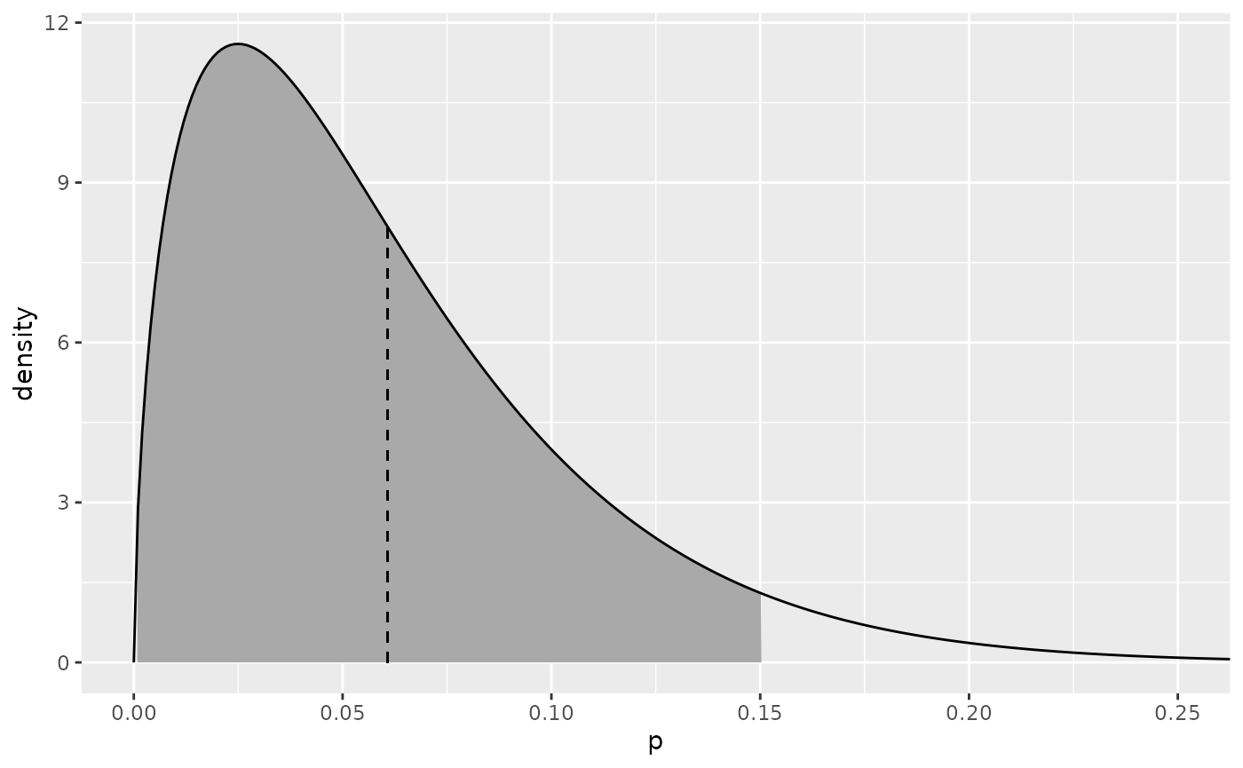
When describing a prior distribution, including a generating prior for planning sample size, it is often more useful to start with quantiles than with the distribution’s parameters. For example, we may believe that a probability is centered around 0.05 and has 95% of its mass lower than 0.15. From these quantiles we can estimate corresponding beta parameters.

params <- betaParamsFromQuantiles(q = c(0.05, 0.15), p = c(0.5, 0.95))
params
#> $a
#> [1] 1.612966
#> 
#> $b
#> [1] 24.93702

We can visualize the results by plotting the distribution. Note that the mean and the median of a beta distribution are not the same. We specified the distribution based on the quantiles 0.5 (median) and 0.95. The dashed line in the plot indicates the mean or expected value. If you want parameters that result in a specific mean and a quantile, I suggest experimenting with moving the median around until you get the mean you want.

plotdbeta(params$a, params$b, HDImass = 0.95) +
  coord_cartesian(xlim = c(0, 0.25))
#> Coordinate system already present. Adding new coordinate system, which will
#> replace the existing one.